1. Introduction to Artificial Neural Networks
The concept of Artificial Neural Networks (ANNs) was firstly introduced by McCulloch and Pitts in 1943 (Maier and Dandy, 2000; McCulloch and Pitts, 1943), but it not was until 1986, when Rumelhart et al. developed the backpropagation algorithm, when the use of ANNs became popular (Møller and Moller, 1993; Rumelhart et al., 1986).
ANNs are one of the most used techniques in Artificial Intelligence (AI) (Medina et al., 2004). AI can be defined as the discipline or process by which machines learn by themselves. The purpose of IA is to create machines that work like the human brain and that are able “to think” (Standford University Machine Learning Course). Neural Networks (NNs) try to mimic the human brain with computational elements that emulate the neurons (by elements called nodes) and the unions between them (by transfer functions) (Medina et al., 2004; Standford University Machine Learning Course).
NNs are made of different layers: the input layer in which the known data is introduced into de model; the intermediate layers, known as hidden layers; and the output layer in which the final value searched is obtained. Each layer consists of different units (neurons or nodes) (Medina et al., 2004; Standford University Machine Learning Course) and each one is connected to the following layer by a transfer function. In an ANN the output of the layer i-1 is the input of the layer i. The known data is introduced into the input layer and a bias term is added, then these data are multiplied by an initial weight and summed, this is after transferred through functions to the following layer until the output layer is reached and the final value is obtained (Dixit and Londhe, 2016).
1.1. Transfer functions and types of ANNs
An ANN uses new features that learn from the input and the mapping of the input. To go from one layer of the NN to the next one, transfer functions are used (Standford University Machine Learning Course). The most common transfer functions used in ocean and maritime engineering are presented in Table 1 (Yogitha and Mathivanan, 2018).
Table 1. Most common transfer functions used in ocean engineering problems.
| Function | Expression | Application |
|---|---|---|
| Linear | (1) | Output layers |
| Logistic sigmoid | (2) | Output and hidden layers. Range of values: [0,1] |
| Hyperbolic tangent sigmoid | (3) | Hidden layers |
| Range of values: [-1,1] | ||
| Radial basis | (4) | Output and hidden layers |
The most common type of ANNs is the feed forward multilayer perceptronneural network (FFNN), but there also other network types that proved to perform very well in ocean engineering problems. All these networks are explained below.
The FFNN is the most common NN. It usually has one or more hidden layers of sigmoid neurons followed by an output layer of linear neurons and can be used as a general function approximator (Demuth et al., 1992). The main characteristic of FFNNs is that they only process information in one direction, which means that there are no back connections (Teslyuk et al., 2021). The first step to build a FFNN is to define a network object, inputs and outputs are selected and weighted and then, the NN is trained and validated (Demuth et al., 1992). They are the simplest type of NNs, but usually have lower rates of accuracy and fail to model time-varying processes. They are also very sensitive to initial weights.
The Cascade-Feed-Forward network (CFF) is a NN in which each hidden unit forms one layer that receives connections from the network's original inputs and the pre-existing hidden units. (Qiao et al., 2016).Therefore, the only difference between a CFFNN and a common FFNN is that each neuron layer is related to all next neuron layers and these additional connections might improve the speed at which the network learns, although the complexity of the NN increases (Pashova and Popova, 2011).
The Feed-Forward Time Delay network (FFTD) is a special feed-forward network with a tapped delay line at the input data set that is introduced to generate dynamics in the static structure. Therefore, FFTDs are used to model dynamic systems and time-varying processes (Yazdizadeh and Khorasani, 2002). Each delay is associated with a weight and its purpose is to provide the network with the capability of representing the relationships between events in time (Pashova and Popova, 2011). The output at time “t” are summed with the outputs at time “t-1”, “t-2”, etc., allowing the creation of richer and more complex decision surfaces (Menezes and Barreto, 2008). Another difference between the FFTD and the FFNN is in the number of branches that connect any two neurons. In the FFNN, generally, there is only one branch connecting any two neurons, whereas in the FFTD more than one branch may be used (Yazdizadeh and Khorasani, 2002).
The radial basis function (RBF) NN is a network that only uses one hidden layer, the output units form a linear combination of the basis functions computed by hidden units and the basis functions in the hidden layer produce a localised response to the input (Evans et al., 2000). It is segmented in two phases. In the first phase, unsupervised learning of the input information is conducted, it classifies information into clusters, that are used in the second phase to yield the output after a supervised learning process is done (Kalra et al., 2005a). The training phase in a RBF NN consists of finding the centres, widths, and the weights connecting hidden nodes to the output nodes. This not only is more efficient, but can sometimes model the data non-linearities in a better way. Their main problem is that they are highly dependent on the choice of centres and width (Evans et al., 2000).
The General Regression Neural Network (GRNN) is a kind of the radial basis network that is often used for regression problems (Pashova and Popova, 2011). It is a nonlinear RBF NN based on nonparametric estimation (Ding et al., 2013). These networks are composed of a RBF layer and a linear layer and they are based on kernel (nonlinear) regression. As its name indicates, this function is capable of approximating any arbitrary function from historical data and it does not require any iterative training process, it draws the estimation functions directly from the training data (Su et al., 2011). They usually have a higher degree of forecasting accuracy and performs statistically better (Leung et al., 2000). Its main problem is that they do not perform well extrapolating.
The adaptive neuro-fuzzy inference system (ANFIS) is another type of NN that consists of an hybrid scheme which uses the learning capability of the ANN to derive the fuzzy if-then rules. The difference between the common NN and the ANFIS is that while the former captures the underlying dependency in the form of the trained connection weights, the latter does so by establishing the fuzzy language rules (Kalra et al., 2005a). This type of ANN has two main parts called as premise and consequence parts and the training in ANFIS consists of determining the parameters belonging to these parts with an optimization algorithm. It eliminates the disadvantage of ANNs of assigning arbitrary weights without explanation (Karaboga and Kaya, 2019).
Recurrent networks (RNNs) are NNs with internal loops that introduce delayed-activation dependencies across the units of the network (Marhon et al., 2013). The main difference with FFNNs is that in FFNNs the signal is passed only in a forward direction, whereas in RNNs the output obtained is fed back into the network through the input layer (Gopinath and Dwarakish, 2015). Connections between nodes form a time-oriented graphs that allows to exhibit dynamic behaviour over time (Teslyuk et al., 2021), this is the main advantage with respect to other networks, they can represent time-varying processes (Marhon et al., 2013). In addition, they usually perform better when the data is noisy, but they can have difficulties in capturing long-term dependencies because the influence of a given input decays exponentially as it cycles around the network's recurrent connections (vanishing gradient problem). This can be solved including inputs at explicit time lags (NARX networks) or with Long short-term memory (LSTM) NNs (Maier and Dandy, 2000; Graves and Graves, 2012).
Long short-term memory (LSTM) neural networks are developed based on the previously explained RNNs. Instead of the neurons of a conventional NN, they have long and short-term memory cells and forget and outputs gates to write, read and reset operations for the cells (Graves and Graves, 2012; Gao et al., 2021). These gates allows the LSTM NN to store information for a long period of time if it is required, which ends with the vanishing gradient problem. The main advantage with respect to RNNs is that they can be used to classify, process, or predict time series when there are time delays of unknown duration between important events and that they can save information in any length of time (Marhon et al., 2013). LSTM NNs use historical information to assist with current decisions and, through the mechanism of a forget gate, they can choose to remember or forget long-term information (Fan et al., 2020). Lara-Benítez et al. proved that they are one of the best alternatives (Lara-Benitez et al., 2021).
Determining the ANN architecture is another difficult task. More complex networks usually model processes more accurately, but are also more expensive and may have problems in generalisation (Maier and Dandy, 2000).
1.2. Training algorithms
Before an ANN is used for forecasting it has to be trained. The most common procedure is to use the 70–80% of the data to train the network and the remaining 20–30% to test its performance. There are many different training algorithms of which the most common is the backpropagation algorithm (Mandal and Prabaharan, 2006). In this section the most popular algorithms are presented.
1.2.1. Gradient descent algorithms
Error backpropagation (BP): It is called backpropagation algorithm because the error is propagated back to update the weights and the biases using an optimization technique (gradient descent), which minimizes the error (Dixit and Londhe, 2016). The backpropagation propagates the input forward through the network and the sensitivities backward, it updates the network weights and biases in the direction in which the performance function decreases most rapidly, which is the negative of the gradient. Its main drawbacks is that it is a local algorithm, which means that it can reach a local optimum instead of the global optimum, and that it is slow in converging (Demuth et al., 1992; Hagan et al., 1996).
It also exists the variant gradient descent with momentum (GDM), which objective is to faster the convergence of the algorithm. The momentum smooths the oscillations of the algorithm and allows the network to respond not only to the local gradient, but also to recent trends in the error surface, avoiding getting stuck in a local optima (Demuth et al., 1992; Hagan et al., 1996).
One of the main problems of the conventional backpropagation algorithm is that it is too slow. Therefore, there are other algorithms known as “faster training” that avoids this problems (Demuth et al., 1992):
Resilient backpropagation (RBP): ANNs usually use sigmoid functions in the hidden layers. These functions transform values from an infinite range to a range of 0–1 and of −1 to 1. This can cause the gradient to have a very small magnitude, which can cause small changes in the weights and biases, generating problems when using the gradient descent technique. The objective of this algorithm is to avoid these effects by determining the weights and bias by a separate update value (Demuth et al., 1992).
1.2.2. Conjugate gradient (CG) algorithms
Conjugate gradient descent algorithms are also classified as “faster training”. Common gradient descent updates the network weights and biases in the direction in which the performance function decreases most rapidly, which is the negative of the gradient. However, this does not necessarily produce the fastest convergence. Conjugate gradient algorithms also search along conjugate directions. There are different conjugate gradient functions (Demuth et al., 1992; Hagan et al., 1996):
-
-
Fletcher-Reeves (CGF): It computes the previous search direction by multiplying it by a factor that is the ratio of the norm squared of the current gradient to the norm squared of the previous gradient. It guarantees to locate the minimum of any quadratic function of n arguments in at most niterations (Demuth et al., 1992; Fletcher and Reeves, 1964).
-
-
Polak-Ribiére (CGP): In this case the factor is the inner product of the previous change in the gradient with the current gradient divided by the norm squared of the previous gradient (Demuth et al., 1992; Fletcher and Reeves, 1964).
-
-
Powell-Beale Restarts (CGB): In common conjugate gradient descent algorithms search direction will be reset to the negative direction of the gradient when the number of iterations is equal to the number of network parameters. The CGB technique restarts the direction of searching to the negative of the gradient if there is very little orthogonality left between the current gradient and the previous gradient (Demuth et al., 1992; Powell, 1977).
-
-
Scaled conjugate gradient descent (SCG): All previous functions use line search, which is computationally expensive. Instead of the line search approach, the SCG uses the model-trust region approach (used in the Levenberg-Marquardt algorithm) to scale the step size and combines it with the conjugate gradient approach (Møller and Moller, 1993; Demuth et al., 1992).
1.2.3. Quasi-Newton's algorithms
Newton's algorithms usually converge faster than gradient methods, but they are much more computationally expensive because they have to compute the Hessian matrix. Quasi-Newton's algorithms are based on Newton's method, but do not require calculation of second derivatives. There are two main algorithms (Demuth et al., 1992):
-
-
Broyden, Fletcher, GolFarb and Shanno (BFGS): It is based on conjugate directions combined with line search. It requires more computation in each iteration and more storage than the conjugate gradient methods, although it generally converges in fewer iterations. It is especially appropriate for small networks (Møller and Moller, 1993; Demuth et al., 1992).
-
-
One step secant algorithm (OSS): It deals with the problem of the storage needed for the BFGS algorithm. This algorithm assumes that at each iteration, the previous Hessian was the identity matrix (Demuth et al., 1992).
1.2.4. Levenberg-Marquardt algorithm (LM)
It is a variation of Newton's method that was designed for minimizing functions that are sums of squares of other nonlinear functions. When the performance function has the form of a sum of squares the Hessian matrix can be approximated as the product of the Jacobian matrix, that is much less complex than computing the Hessian matrix (Demuth et al., 1992; Hagan et al., 1996).
ANNs can perform very well in the training data set, but fail to perform in the test data set, which means that they do not perform well when adding new data. When the ANN is not able to generalize the problem is known as “overfitting”. This problem can be solved using regularization or early stopping (Standford University Machine Learning Course; Hagan et al., 1996). Regularization is a technique in which the different features are penalized by multiplying it by a factor λ, smoothing the function and making the network less complex (Standford University Machine Learning Course). One of the most common regularization techniques used in ocean engineering is the Bayesian regularization (BR). Mackay (1992) was the first one in applying the Bayesian framework to ANN modelling.
2. ANNs in ocean engineering
Numerical models are the most common used approach to solve ocean and maritime engineering problems. However, with the development of machine learning it has been showed that ANNs are a very good alternative to this traditional approach, they even give better results, especially when the problem is random and includes non-linear patterns (Fan et al., 2020). The differences in the modelling approach between ANNs and traditional statistical models is that the former couple with a lack of strict governing rules, which makes them ideal for problems with a random distribution of variables (Maier and Dandy, 2000).
In ocean engineering ANNs have been used since 1995, Mase (1995) was the first one to use them to evaluate the artificial armour layer stability of a breakwater. Since then, ANNs have been widely used. In this paper the following fields of ocean engineering in which ANNs have been applied are distinguished: prediction of wave heights, prediction of the water level, tides, extremes and wave energy and application to ports, pipes and breakwater stability.
2.1. Prediction of wave heights
One of the main applications of ANNs is to predict wave heights, prediction of waves is an uncertain and random process that makes it ideally suited to NN modelling (Deo et al., 2001).
Deo and Naidu were the first authors that proved the advantages of ANNs over traditional methods for wave-height forecasting in 1998 (Deo and Sridhar Naidu, 1998). In 2001 Deo et al. predicted significant wave heights and average wave periods from the input of wind speeds (Deo et al., 2001). In 2002 Agrawal and Deo did it from current and previous wave heights (Agrawal and Deo, 2002). They found that when shorter prediction intervals are concerned, the NN had distinct superiority over the stochastic approach. However, this was not the case when a longer interval of prediction was studied. One year later, Deo and Jagdale showed that ANNs could also be used to predict breaking wave heights (Deo and Jagdale, 2003). In 2004 Agrawal and Deo concluded that ANNs outperformed more the statistical regressions when the input–output structure to be established is hazier and more unclear (Agrawal and Deo, 2004).
Also in 2004 Makarynskyy studied how to improve wave predictions with ANNs (Makarynskyy, 2004). A separate NN was developed to forecast each wave parameter at every location. One year later Makarynskyy et al. did a similar study with two approaches (Makarynskyy et al., 2005). They first used one ANN for each parameter (wave height and period) and in the second approach they used a unique ANN to predict both. They proved that the simplification of the NN sometimes gave better results. In 2005 Karla et al. conducted another two research. In the first one, they used satellite data and saw that this data needed pre-processing before applying it to ANNs (Kalra et al., 2005a). In the second one they also translated offshore satellite wave data and proved that the RBFNN performed better than the FFNN, but for higher waves the FFNN was more accurate (Kalra et al., 2005b).
In 2008 Jain and Deo conducted an experiment on AI tools to forecast waves in real time (Jain and Deo, 2008). They applied ANNs, genetic programming and model trees and saw that the differences between these 3 techniques were negligible. This same year Malekmohamadi et al. compared the performance of numerical wave modelling (NWM), ANNs and an hybrid model (Malekmohamadi et al., 2008). They concluded that although the NWM leaded to better results, such models were computationally expensive and needed long-time execution. Using artificial patterns for training ANNs leaded to more acceptable results, than those obtained using observed patterns. Also in 2008 Günaydin compared seven different ANN models with traditional regression methods (Gunaydin, 2008). They showed that the best performance was given when all the meteorological factors were included as inputs. Between all the meteorological inputs, wind speed was the most effective. The same year Mahjoobi et al. applied ANNs, Fuzzy Inference Systems (FIS) and ANFIS (Mahjoobi et al., 2008). They implemented a separate network for each parameter, and after one network for the three output variables. Results indicated negligible differences between the two approaches.
In 2009 Tsai and Tsai used ANNs to convert the signal of pressure transducersinto significant wave height, wave period, maximum wave height, and spectral peakedness (Tsai and Tsai, 2009). They compared the results with the ones obtained applying a linear wave pressure transfer function and found that for water depths greater than 20 m the NNs worked significantly better.
In 2015 other authors, Gopinath and Dwarakish proved that NARX models needed less data than conventional NNs to obtain the same results (Gopinath and Dwarakish, 2015). In 2016 Londhe et al. used ANNs to predict the errors in wave forecasting and added or subtracted these errors from the valued predicted by the numerical model, improving their predictions (Londhe et al., 2016). Salah et al. discovered that the hybrid model that combined SWAN and ANNs models outperformed both approaches, traditional and soft-computing (Salah et al., 2016). In 2017 Abhigna et al. saw that to predict extreme values of wave heights (both, high and low) ANNs performed worse (Abhigna et al., 2017). This same year Mudronja et al. stated that ANNs outperformed more traditional models when the number of inputs involved was high (Mudronja et al., 2017) and Sadeghifar et al. proved that the use of NARX networks improved the prediction of wave heights (Sadeghifar et al., 2017).
In 2020 Vieira et al. used ANNs to fill the gaps in wave records (Vieira et al., 2020). The inputs were wave and wind parameters. They performed several FFNNs with 3 (wave parameters) and 5 inputs (wave and wind parameters) and concluded that wind was not and essential parameter in that case, contrary to other studies. This same year, Stavarache et al. studied how to optimize ANNs for wave prediction and proposed to substitute the traditional trial and error approach by genetic algorithms (Stavarache et al., 2020). In 2021 Gao et al. concluded that LSTM networks had several advantages with respect to other soft-computing and conventional models (Gao et al., 2021). They also highlighted that a higher number of hidden neurons did not necessarily imply better results and that this number had to be adjusted to each wave height. This results were in line with Jörges et al. (Joerges et al., 2021).
In 2022 Sadeghifar et al. conducted an study in which they compared the performance of different soft-computing techniques (ANNs, ANFIS, Random Forest and M5P models) and proved that the M5P outperformed the others (Sadeghifar et al., 2022).
The studies presented in this section are summed up in Table 2.
Table 2. Wave height studies.
| Author | NN type | Architecture | Algorithm | Performance evaluation | Training and test |
|---|---|---|---|---|---|
| Deo and Sridhar Naidu (1998) | FFNN | 1-5-1 | BP | Global errorTime Nºiterations | 80% and 20% |
| 1-2-1 | CG | ||||
| 1-0-1 | Cascadea | ||||
| Deo et al. (2001) | FFNN | 2-4-2 4-4-4 | BP, CG and Cascade | R | 80% and 20% |
| Agrawal and Deo (2002) | FFNN | – | BP, CG and Cascade | Correlation coefficient (R) Root mean square error (RMSE) | 80% and 20% |
| Deo and Jagdale (2003) | FFNN | 3-5-5-2 | BP | R, Maximum, minimum and average error | – |
| Agrawal and Deo (2004) | FFNN | – | BP and Cascade | R, RMSE | 80% and 20% |
| Makarynskyy (2004) | FFNN | 48-97-24 | RBP | R, RMSE, SI | 52% and 48% |
| Kalra et al. (2005a) | RBF | 21-13-1 | RBF | R, RMSE, Mean absolute error (MAE), Scatter index (SI), Mean square relative error (MSRE) | 80% and 20% |
| FFNN | 21-9-1 | BP, SCG, CGB, BFGS, LM | |||
| ANFIS | – | – | |||
| Kalra et al. (2005b) | FFNN | 27-9-1 | RBP, SCG, CGB, BFGS, LM | R, RMSE, MAE | 70% and 30% |
| RBF | 27-3-1 | RBF | |||
| Makarynskyy et al. (2005) | FFNN | 8-17-1 | BP, RBP, LM | R, RMSE, SI | – |
| 4-9-1 | |||||
| 2-5-1 | |||||
| 6-17-4 | |||||
| 12-21-5 | |||||
| Jain and Deo (2008) | FFNN | 4-4/5-1 | LM | R, RMSE, MAE | 60% and 40% |
| Malekmohamadi et al. (2008) | FFNN | 8-8-1 | BP | R, Total error | – |
| Hybrid model | 24-24-1 | BP | |||
| Gunaydin (2008) | FFNN | 3-2-1 | LM | R, Mean Square Error (MSE) and Mean Absolute Relative Error (MARE) | 80% and 20% |
| Mahjoobi et al. (2008) | FFNN | 4-7-1: Period and height | BP | R, SI, MSE, MSRE, BIAS | – |
| 4-11-1:Dir log | |||||
| 4-8-1:Dir tan | |||||
| 4-9-3 | |||||
| ANFIS | – | – | |||
| Tsai and Tsai (2009) | FFNN | 4-8-2 | BP | R, Root Mean Square Deviation (RMSD) | 75% and 25% |
| Gopinath and Dwarakish (2015) | FFNN | 52-10-52 | LM | R, MSE, RMSE, Sum Squared Error (SSE) | – |
| 12-5-12 | |||||
| NARX | 1-6-25 | – | |||
| 1-10-12 | |||||
| Salah et al. (2016) | FFNN | 10 hidden nodes | SCG, LM | R, RMSE, SI, BIAS | 80% and 20% |
| Londhe et al. (2016) | FFNN | 9-1-1 | LM | R, MSE, MAE, RMSE, SI, BIAS, Coefficient of efficiency (CE) | 70% and 30% |
| 4-1-1 | |||||
| 9-8-1 | |||||
| Abhigna et al. (2017) | FFNN | – | CG, LM, BR | R, MSE | – |
| Recurrent NN | |||||
| Mudronja et al. (2017) | FFNN | 1- [10 to 50]-1 | LM, BR | RMSE, MAE, CE, Percent BIAS, Standard Deviation Ratio (RSR) and Persistency Index (PI) | – |
| 2-[10 to 50]-1 | |||||
| Vieira et al. (2020) | FFNN | 3-[4/8/12]-1 | LM, BR | R, RMSE, SI, BIAS | 70% and 30% |
| 5-[4/8/12]-1 | |||||
| Stavarache et al. (2020) | FFNN | 5-5-9-8-1 | LM, Quick Propagation | R, RMSE | – |
| Gao et al. (2021) | LSTM | Several | BP | R, RMSE, SI MAE | – |
| Joerges et al. (2021) | LSTM | – | – | R, RMSE, MAE, Mean Arctangent Absolute Percentage Error (MAAPE), Coefficient of Determination R2 | 70% and 30% |
| Sadeghifar et al. (2022) | FFNN, ANFIS | 4-10-1 | – | R, RMSE, MAE, SI, BIAS, CE | 70% and 30% |
- a
-
The algorithms and networks in bold were the ones that performed the best.
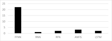
From all the type of networks, the FFNN was clearly the most used. Although in the last years LSTM neural networks are giving promising results (Fig. 1).
 Fig. 1. Frequency of networks used in wave height ANNs studies.
Referring to the architecture of the studies, all of them excepted one opted for a 3-layer neural network because adding more layers did not result in a significant improvement. In ocean engineering, shallow ANNs with one hidden layer are enough to forecast wave-heights. The number of inputs and outputs depends on the physics of the problem and has to be studied in each case. The number of hidden neurons also depends on the problem and its level of complexity. All of them were usually optimized by trial-and-error analysis.
From all the algorithms presented, the BP and the LM were the most used to predict wave height. The efficiency of each algorithm depended on the characteristics of the problem. To choose the best algorithm, each case has to be studied (Fig. 2).
 Fig. 2. Frequency of algorithms used in wave height ANNs studies.
With respect to the error measures, 22 out of 24 studies used the correlation index (R) as one of the main variables to optimize the network, 65% of the studies also used the RMSE, and the rest of statistics to quantify the performance of the NN depended on the study and on the authors choice.
2.2. Prediction of water level, tides, extremes and wave power
ANNs have also been used in ocean engineering to predict water level, tides and wave power. Tsai and Lee were one of the first ones to use ANNs to predict tides in 1999 (Tsai and Lee, 1999). Lee et al. also used it two years later, they tried different networks with 0, 1 and 2 hidden layers and concluded that the best performance was given by one hidden layer with BP algorithm (Lee and Jeng, 2002; Lee et al., 2002). In 2004 Lee conducted a similar study, but he did it to predict long-term tides, they proved that ANNs were as accurate as traditional harmonic analysis and needed less data (Lee, 2004). In 2006 Chang and Lin compared the ANN results with the NAO.99b model and concluded that both methods were accurate and that the NNs could be applied to different locations with similar tide type (Chang and Lin, 2006).
In 2008 Liang et al. performed one-step and multistep methods, concluding that the last one was better to predict water levels (Liang et al., 2008). This same year, Han and Shi predicted water levels and pointed out the usefulness of this technique not only for short-term forecasts, but also for long-term (Han and Shi, 2008). Next year, de Oliveira and Ebecken used a RBF NN and a GRNN to predict sea level and surge. The results indicated that NNs could also be useful as a complement for the standard harmonic model (de Oliveira and Ebecken, 2009).
In 2010 Wenzel and Schröter used ANNs with two main purposes: filling data gaps in the tide gauge time series and estimating the evolution of regional mean sea levels from these tide gauge data (Wenzel and Schroeter, 2010). Next year, Pashova and Popova compared the performance of five different neural networks on predicting water level and concluded that the best performance was given by the FFNN with LM, LM algorithm was the fastest, and BFGS gave the best results in most cases (Pashova and Popova, 2011). In 2012 Filippo et al. also concluded that ANNs were a very interesting tool to predict water levels and also to complement traditional harmonic analysis approach (Filippo et al., 2012). In 2014 Karamouz et al. used two innovative models called ELMAN (special type of the common FFNN with context units) and IDNN (type of FFTD) for sea-level simulation and saw that sea surface temperature was an important variable to consider (Karamouz et al., 2014). This same year Kusnandar et al. estimated the mean sea level change by hybridizing exponential smoothing and a NN, which gave promising results (Kusnandar et al., 2014). Castro et al. also studied the wave energy potential in nearshore coastal areas using ANNs and saw that the most important variable to do these predictions was the wave-height (Castro et al., 2014).
In 2015 El-Diasty and Al-Harbi compared the performance of an ANN; traditional harmonic analysis and a wavelet network, which is an algorithm that connects the NN with the wavelet decomposition. Results showed that the wavelet network was the most accurate (El-Diasty and Al-Harbi, 2015). In 2018 El-Diasty et al. did another research using wavelet technique, but this time hybridizing it with the harmonic analysis technique, which gave even better results (El-Diasty et al., 2018). In 2019 Zhao et al. applied different ANNs to forecast sea level anomalies, they predicted sea level variation with the least-square fitting methodology and the stochastic residual terms with different NN models. They found that this hybrid approach gave results with relatively high precision (Zhao et al., 2019).
Wang et al. also used wavelet networks to predict tides and sea water level (Wang et al., 2020a, 2020b, 2020c). In 2020 they combined wavelet decomposition and ANFIS models for predicting multi-hour sea levels and highlighted the advantages of these hybrid models (Wang et al., 2020c). After, they improved wavelet networks adding a momentum term (Wang et al., 2020a). This same year, they also improved wavelet networks using a genetic algorithm to optimize the weights and parameters of the NN (Wang et al., 2020b). All these models performed significantly better than the traditional harmonic analysis. In 2020 Avila et al. used Fuzzy systems and ANNs to predict wave energy and both models gave very accurate results without needing a base data of many years (Avila et al., 2020). In this same year Bruneau et al. studied sea level extremes with a deep NN, they used a total of 600 tide gauges around the world to predict the non-tidal residual as well as extremes events and concluded that ANNs outperformed predictions based on multivariate linear regressions (Bruneau et al., 2020).
In 2021 Primo de Siqueira and Paiva used a combined approach of process-based and data-based model to improve the forecasting of sea levels, they used the process-based model to forecast the linear part and the ANNs to forecast the non-linear part and the results obtained were significantly better (Primo de Siqueira and Paiva, 2021). Yang et al. used deep neural networks (NNs with more than two hidden layers) to predict tides and analysed the effects of gaps in data records, they concluded that, among all the methods, deep neural networks performed the best (Yang et al., 2021). Bai and Xu compared RBF and LSTM NNs with an innovative approach: bidirectional LSTM NNs, that is a LSTM NN that combines the information for both, front and back directions of time series, and proved that was the best option (Bai and Xu, 2021). Bento et al. concluded that in the case of extreme unforeseen events (long-term forecasts), the DNN presented a slightly underestimated time-series prediction and more data was needed. The errors of DNNs also depended on the seasonality, winter forecasts were less accurate than summer forecasts due to its greater variability (Bento et al., 2021).
The studies presented in this section are summed up in Table 3.
Table 3. Sea level, extremes and energy studies.
| Author | Network type | Architecture | Algorithm | Performance evaluation | Training and test |
|---|---|---|---|---|---|
| Lee and Jeng, 2002 | FFNN | 4-4-1 | BP | RMSE | – |
| Lee et al. (2002) | FFNN | 138-7-69 | BP | R, RMSE | – |
| Lee (2004) | FFNN | 138-7-69 | BP | R, RMSE | – |
| Chang and Lin (2006) | FFNN | 5 hidden neurons | LM | R, RMSE | – |
| Han and Shi (2008) | FFNN | 3 layers, 10 neurons | LM | R, RMSE, SI | – |
| Liang et al. (2008) | FFNN | 50 hidden neurons | BP | R, RMSE | – |
| de Oliveira and Ebecken (2009) | RBF | 7-9-1 | BP for FFNN | R, RMSE, R2 | 50% and 50% |
| FNN | 7-11-1 | ||||
| GRNN | 7–14–1 | ||||
| Wenzel and Schroeter (2010) | FFNN | 112-84-56 | BP | RMSE | – |
| Pashova and Popova (2011) | FFNN, CFF, FFTD, RBF, and GRNN | 11-6-1 | BP, LM, RBP, BFGS | R, RMSE, SI, R2 | 79% and 21% |
| Filippo et al. (2012) | FFNN | 4 inputs | BP | R, Regression Ratio, Error | |
| 1 output | |||||
| Karamouz et al. (2014) | FFNN | 1 to 20 hidden neurons | BP | RMSE, Volume Error Percent (VE) | – |
| ELMAN (FFNN) | 19 hidden neurons | LM | |||
| IDNN (FFTD) | 17 hidden neurons | BP | |||
| ANFIS | – | – | |||
| Castro et al. (2014) | FFNN | 3-4-4-1 | BP | R, MSE and Normalized MSE (NMSE) | 2/3 and 1/3 |
| El-Diasty and Al-Harbi (2015) | ANN | 24-12-1 | BP | R, RMSE, MAE, Maximum Absolute Error, Percentege of RMSE | 80% and 20% |
| Wavelet | |||||
| El-Diasty et al. (2018) | Hybrid wavelet | 24-12-1 | – | R, RMSE, MAE,Model error at 95% | 80% and 20% |
| Zhao et al. (2019) | GRNN | 5-0.25-1 | RBF | R, RMSE | – |
| FFNN | 5-20-15-1 | BP | |||
| RBF | 5-20-1 | RBF | |||
| Wang et al. (2020c) | Wavelet | 3 layers | LM | RMSE, MAE, MSRE, CE | 80% and 20% |
| ANFIS | |||||
| Wavelet+ANFIS | |||||
| Bruneau et al. (2020) | FFFNN | 33-48-48-48-1 | – | MSE, MAE | 2/3 and 1/3 |
| LSTM | – | ||||
| Avila et al. (2020) | FFNN | Input-15-1 | GMS, RBP | R, MAE, Mean Relative Error | 89% and 11% |
| Primo de Siqueira and Paiva (2021) | FFNN | 10 hidden neurons | LM | R, RMSE | 75% and 25% |
| Bento et al. (2021) | FFNN | MFO iterations | SCG | R, RMSE, MSE, Mean Absolute Log-difference Error (MALE) | 75% and 25% |
| Bai and Xu (2021) | FFNN, RBF, Bi-LSTM | 80/200 memory cells | BP for FFNN | R, RMSE, MSE, MAE, R2 | – |
| Yang et al. (2021) | FFNN | –a | BP | RMSE, MAPE | 50–90% and 50-10% |
- a
-
The algorithms and networks in bold were the ones that performed the best
From all the type of networks, the FFNN was clearly the most used. Although in the last years wavelet neural networks are getting more popular (Fig. 3).
 Fig. 3. Frequency of networks used in sea level, energy and extremes ANNs models.
Referring to the network architecture, the conclusions are the same as in Section 2.1.
From all the algorithms presented, the BP was the most used to predict sea level. The efficiency of each algorithm depended on the characteristics of the problem. However, LM algorithm seemed to be the most effective basing on the studies above presented, the majority of them selected the LM algorithm after proving that it was the most effective (Fig. 4).
 Fig. 4. Frequency of algorithms used in sea level, energy and extremes ANNs models.
With respect to the error measures, 18 out of 22 studies (which means more than the 80% of the studies) used the correlation coefficient and the RMSE as the main statistical variables to evaluate the performance of the model.
2.3. Application to breakwaters, ports and pipes
One of the first applications of ANNs to maritime and ocean engineering was to study breakwater stability and one of the first authors to do it was Mase, who in 1995 used a 3-layer FFNN to estimate the artificial armour layer stability (Mase, 1995; Mase et al., 1995).
In 2005 Yagci et al. used ANNs and fuzzy logic and saw that ANNs can be employed successfully to estimate the breakwater damage ratio (Yagci et al., 2005). This same year Kim and Park compared the performance of 5 different ANNs for stability prediction (Kim and Park, 2005). They concluded that any NN became more effective when using the design parameters as independent network input rather than using artificial parameters. In 2014 Kim et al. highlighted the convenience of including tidal level in this type of studies to not overestimate breakwater damage (Kim et al., 2014).
In 2008 Iglesias et al. developed a virtual laboratory to estimate breakwater stability (Iglesias et al., 2008). They called the model “a virtual laboratory” because it was capable of estimating the damage caused to a rubble-mound breakwater by waves like a conventional laboratory would do. Two years later, Balas et al. studied breakwater stability with ANNs, fuzzy systems, ANFIS models and ANNs with Principal Component Analysis (PCA) and highlighted that hybrid models performed better than conventional ANNs and captured better nonlinearities (Balas et al., 2010). In 2012 Koç and Balas conducted a similar study in which they used genetic algorithms (GA) and fuzzy NNs, and pointed out that hybrid models needed less data samples (Koç and Balas, 2012). In 2011 Akoz et al. stated that ANNs were an important tool that can be applied for the design of coastal structures under the action of most critical loading (Akoz et al., 2011). In 2013 Suh et al. combined this soft-modelling technique with SWAN model to reduce the computation time and analysed the effects of seal level rise and wave height increase on caisson sliding (Suh et al., 2013).
Referring to application of ANNs to ports studies, one of the most important authors are López and Iglesias, who in 2013 and 2015 conducted two different studies to estimate energy and operability conditions in a harbour (López and Iglesias, 2013, 2015). In 2013 they estimated the amount of energy inside the harbour and they used two different NN models, one that directly estimated the energy and another model that did it in two steps. They concluded that ANNs constitute a valid, efficient approach for estimating wave energy inside or outside a harbour and that the direct approach outperformed the model with two steps (López and Iglesias, 2013). To assess harbour operability, they followed a similar methodology and stated that one-hidden layer NN performed better than 2-hidden layer NN for this case, they also carried a sensitivity analysis and saw that wave height and period were the two variables which most influenced wave agitation (López and Iglesias, 2015).
Previous to these studies Londhe and Deo conducted a research on wave tranquillity inside a harbour (Londhe and Deo, 2003). They used different training algorithms: GDM, RP, CGF, CGP, CGB, SCG, BFGS, OSS, and LM. All the algorithms gave satisfactory results. The CGF algorithm was more memory efficient and the SCG algorithm required the minimum time to train. Kankal and Yüksek. also assessed harbour tranquillity using NNs; they studied the effect of different wave parameters, estimated wave height in the harbour basin and optimized the port layout (Kankal and Yüksek, 2012). In 2020 Zheng at al. used ANNs to estimate waves inside a port and compared it with Boussinesq model performance, they trained the network using numerical models and validated it with observations, proving that ANNs are an efficient tool to forecast wave parameters (Zheng et al., 2020).
In addition, in the last months (March and April 2022) Moslemi et al. have published two articles about the thermal response in pipes containing fluid and gas which has a great application in ocean engineering (Moslemi et al., 2022a, 2022b). In the first study (Moslemi et al., 2022a) they used ANNs to determine the temperature and phase change rate in the extrusion process, they compared the experimental and numerical results and concluded that numerical results can be used in ANNs training and that ANNs can be used to optimize the parameters of additively manufactured polymers used in ocean pipelines. In the second study (Moslemi et al., 2022b) they applied a FFNN to determine the correlation between the welding pool characteristics as input and the Goldak parameters as output and concluded that ANNs outperform regression models, but they are more complex.
The studies presented in this section are summed up in Table 4.
Table 4. Breakwater and ports studies.
| Field | Author | Network type | Architecture | Algorithm | Performance evaluation | Training and test |
|---|---|---|---|---|---|---|
| Breakwaters | Mase et al. (1995) | FFNN | 6-12-1 | BP | MSE | – |
| Yagci et al. (2005) | FFNN | 5-3-1 | BP | MSE | 75% and 25% | |
| RBF | ||||||
| GRNN | ||||||
| Kim and Park (2005) | FFNN | [5-7]- 4/5/20- 1 | BP | Index of agreeement | – | |
| Iglesias et al. (2008) | FFNN | 4-9-8-7-6-5-1 | BP | MSE | 2/3 and 1/3 | |
| Balas et al. (2010) | FFNN | 5-4-1 | GDM | R, MSE | 80% and 20% | |
| ANN with PCA | 5-4-1 | 54% and 46% | ||||
| ANFIS | 10-8-1 | – | ||||
| Akoz et al. (2011) | FFNN | 4-3-3 | LM | MSE, MAE, MARE, R2 | 75% and 25% | |
| Koç and Balas (2012) | ANFIS | 2 hidden layers | – | R, R2, Mean Absolute Percentage Eror (MAPE), CE | – | |
| Hybrid (GA) | 5 inputs and 1 ouput | GA and Climbing Hill | 38% and 62% | |||
| Suh et al. (2013) | FFNN | 5 to 60 hidden neurons | LM | MSE, Maximum Relative Error (MRE) | 70% and 30% | |
| Kim et al. (2014) | FFNN | 2-3-1 | BP | RMSE | – | |
| Ports | Londhe and Deo (2003) | FFNN | Module networks [3/4-1-1] | GDM, RP, CGF, CGP, CGB, SCG, BFGS, OSS, and LM | MAE, RMSE, MSRE, MRE, R2, CE, Average error (AE) | 80% and 20% |
| Kankal and Yüksek (2012) | FFNN | 5 inputs 24 outputs. 1–2 hidden layers | BP | Average relative error | 80% and 20% | |
| López and Iglesias (2013) | FFNN | 3-2-2-1 | BP, BR | R, MSE | – | |
| 3-3-1 | ||||||
| 2-2-1 | ||||||
| López and Iglesias (2015) | FFNN | 15-57-1 | LM, BR | MSE, RMSE, Normalized RMSE | – | |
| Zheng et al. (2020) | FFNN | 3-7-8-24 | LM, GDM | R, MAE, Relative MAE | 85% and 15% | |
| Pipes | Moslemi et al., 2022a, Moslemi et al., 2022b | FFNN | 5-7-5 | LM | R, MAE, RMSE | 80% and 20% |
| FFNN | 3-3-3-3-4 | LM | R, MAE, RMSE | 70% and 30% |
From all the type of networks, the FFNN was clearly the most used (Fig. 5).
 Fig. 5. Frequency of networks used in breakwaters, ports and beaches ANNs models.
Referring to the network architecture, the conclusions are the same as in Section 2.1 Prediction of wave heights, 2.2 Prediction of water level, tides, extremes and wave power.
From all the algorithms presented, the BP, LM and Conjugant Gradient algorithm were the most used. The efficiency of each algorithm depended on the characteristics of the problem. To choose the best algorithm, each case to be studied (Fig. 6).