1. Introduction and background
Shale is the name for a class of fine-grained sedimentary rocks composed primarily of tiny particles of clay minerals and quartz, the mineral components of mud. These materials were deposited as sediment in quiet water, which was then buried, compacted by the weight of overlying sediment, and cemented together to form a rock through a process called lithification. Clay minerals are a type of sheet silicate related to mica that usually occurs in the form of thin plates or flakes. As the sediment was deposited, the flakes of clay tended to stack one on top of another like a deck of cards, commonly giving lithified shale the property of splitting into paper-thin sheets (Fig. 1). This is called fissility, and it distinguishes shale from other fine-grained rocks like chalk or siltstone(Soeder, 2017).
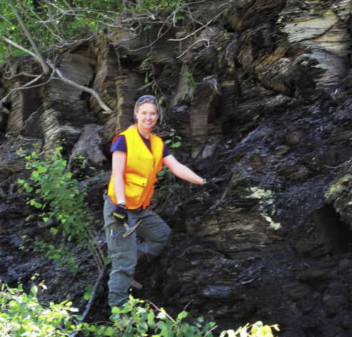
 Fig. 1. SD Mines geological engineering PhD candidate Scyller Borglum at the Marcellus Shale type section near Marcellus, New York. Fissility and vertical fractures are visible behind her. Photo by Dan Soeder, 2016).
Because the grains of material that make up shale are so small, the pore spacesbetween these grains are equally small. Although shale can have porosity in the range of ten percent, the pores and flowpaths are so tiny that it is difficult for any fluids in the pores to move out of the rock (Schieber, 2010, Goral et al., 2015). This is what makes shale so “tight,” requiring the presence of natural and induced fractures for oil and gas (O&G) to flow.
Shale rock comes in dark or light colors depending on organic carbon content (Fig. 2). Dark-colored or “black” shales are organic-rich, whereas the lighter colored “gray” shales are organic-lean. Black shales are the usual targets for unconventional O&G development because of their richer carbon content. Quantitative correlations between organic carbon content and color of the shale have proven impractical, because once the organic carbon content reaches a few percent, the shale is black and doesn't get any darker with the addition of more carbon (Hosterman and Whitlow, 1980). The organic carbon in black shale originated primarily as plant detritus that had accumulated with the sediment, commonly sourced from freshwater algae, marine algae, or terrestrial land plants (Chen et al., 2015). It was preserved by anoxic conditions in the bottom water at the sediment-water interface. The lack of oxygen prevented benthic animals and aerobic decay bacteria from consuming the organic material, thus preserving it in the mud to later form a black shale.
 Fig. 2. Photograph of the contact between the “black” Cleveland Shale and the underlying “gray” Chagrin Shale in a drill core from Ohio, USA. Numbers on the core are depths in feet. Photo by Dan Soeder, 1981).
Along with anoxic bottom waters, two other factors appear to be important for the preservation of organic carbon in sediments: 1) large-scale input of organic material to the water column from algal blooms (Wrightstone, 2011) or other sources at rates faster than it can be consumed while descending to the bottom, and 2) deposition of the organic-rich material in a location with a low influx of clastic sediment, thereby preventing the “dilution” of the organic carbon with large amounts of inorganic minerals (Smith and Leone, 2010). These processes together create organic-rich muds. As these materials were buried deeply beneath younger sediments and subjected to intense heat and pressure over geologic time periods, the organic material evolved into hydrocarbons through a process known as thermal maturation (Rowan, 2006).
There is some debate among geologists concerning the nature of the depositional environment of black shales. One camp proposes that a deepwaterenvironment was required to develop the anoxic conditions necessary to preserve organic matter (Ettensohn, 2012). This so-called “Black Sea” model suggests black shales form as the result of rapid subsidence in a foreland basinbelow the pycnocline. Deep water deposition of black shale is then followed by the infilling of the basin with gray shales and coarser clastics. This concept seeks to explain the alternating sequence of black shales and intervening coarser clastic wedges in places like the northern Appalachian basin as a result of cyclic subsidence caused by mountain building on the basin margin, followed by pulses of coarser sediment entering the basin from the new highlands.
A second school of thought agrees that although the Black Sea model may possibly work in parts of the Appalachian basin and some other geologic settings, many black shales appear to have been deposited on quiet, distal, shallow water platforms under open marine conditions (i.e. Schieber, 1994, Mosher, 2010, Smith and Leone, 2010, Wrightstone, 2011). Petrographic studies often find tiny fragments of fossil skeletal material in black shales from echinoderms, bryozoans, brachiopods, and other benthic animals that would not be expected in deep, anoxic water. This “calci-silt” suggests that the upper layers of sediment were not permanently anoxic, but possibly just seasonally disoxyic (Smith and Leone, 2010), supporting a model for shallow anoxia proposed by Tyson and Pearson (1991), where organic matter from seasonal algae blooms periodically descended to the seafloor, creating anoxic conditions that preserved the organic carbon in the sediment. Smith and Leone (2010) also noted that many black shale units in the Appalachian basin and elsewhere rest on erosional unconformities at the top of the underlying limestones. Formations like the Marcellus Shale, the Rhinestreet Shale, Barnett Shale, Haynesville Shale, Woodford Shale, Pierre Shale, and Bakken Shale all onlap unconformities, suggesting that many black shales were deposited during a distal basin margin transgression onto a surface that may have been eroded during a previous sea level lowstand.
1.1. Hydrocarbon resources in shale
Shale gas hydrocarbon resources are huge. Estimates tabulated by Bruner and Smosna (2011) from different authors on just the Marcellus Shale gas resource range from conservative assessments of about 85 trillion cubic feet (TCF) from the U.S. Geological Survey (Coleman et al., 2011) to more optimistic estimates by Engelder (2009) of nearly 500 TCF of technically recoverable gas. (One TCF equals about 28.3 billion cubic meters). The Utica Shale below the Marcellus may have even greater recoverable reserves in the 750 to 800 TCF range (Hohn et al., 2015). Such estimates are of course built on many assumptions about the formation geology, organic content, gas generating potential, gas in place (GIP), and estimated ultimate recovery (EUR), resulting in a wide range of values (Bruner and Smosna, 2011). A better understanding is needed of the processes that generate and store gas in shale. In nearly all cases, however, the estimates are quite large when compared to conventional gas reservoirs.
In a classic publication, Engelder and Lash (2008) stated that the Marcellus Shale GIP exceeds 500 TCF over an area encompassing parts of New York, Pennsylvania, West Virginia, and Ohio. They assumed a technically recoverable gas fraction of 10%, leading to a reserve estimate of 50 TCF. This caused quite a stir at the time, because 50 TCF of producible gas from a single formation was more than double the annual consumption of natural gas in the United States. More refined calculations by Engelder (2009) came up with significantly higher estimates for GIP, and assuming a power-law decline rate, 80-acre well spacing, and 50-year well life, he predicted a 50 percent probability that the Marcellus Shale will ultimately yield 489 TCF of gas. This is nearly two decades of consumption for the entire United States.
To understand why the gas resources in these shale formations are so large, it may be helpful to review how petroleum and natural gas are created over geologic time periods (Selley, 2014). Rocks that can produce hydrocarbons in commercial quantities with standard well drilling technology are called conventional reservoirs (Soeder, 2017). The hydrocarbons present in a conventional reservoir were usually created elsewhere, and migrated into the reservoir, where they were trapped. Conventional O&G reservoirs are formed by a complicated process that requires a number of events to occur in a specific order. These are: 1) the presence of a source rock containing sufficient preserved organic carbon (generally greater than 2% by weight), 2) burial of the source rock and exposure to high temperatures and pressures over geologic time to “cook” the organic matter in the absence of oxygen, creating natural gas and petroleum, 3) the presence of a porous and permeable reservoir rock above and relatively close to the source rock, 4) a trap and seal on the reservoir rock to contain the hydrocarbons, and 5) development of a migration pathway from the source rock to the reservoir rock so the reservoir can be filled. The rarity of all these things happening with precise timing and in the proper sequence is the main reason conventional O&G resources can often be quite difficult to find. The hunt for structural or stratigraphic traps in potential reservoir rocks above a thermally mature and carbon-rich source rock has kept petroleum geologists busy for decades.
At the other end of the spectrum are shale gas and tight oil, both of which are known as “unconventional” resources (Soeder, 2017). In this case, the shale itself acts as both the source rock and the reservoir rock, representing a new concept in petroleum geology (Charpentier and Cook, 2011). The hydrocarbons present in the shale were created in-place from organic material deposited with the sediment, and remain contained within the fine-grained rock. Thus, unconventional reservoirs can potentially occupy the entire volume of a geological formation without the need for traps and seals, and are known as “continuous resources” (Charpentier and Cook, 2011). They are significantly larger than conventional reservoirs, but they are also much more difficult to develop. In petroleum engineering, the term “unconventional” means that O&G from the target formation cannot be produced in economical amounts using traditional extraction methods, but must be engineered and enhanced with some type of reservoir stimulation technology like hydraulic fracturing (Soeder, 2017).
Why are these resources so large? Plotting the quality of most natural resourcesagainst the quantity typically results in a shape known as the resource triangle (Fig. 3). This shows that the highest-quality resource occurs in small amounts, but significantly greater volumes of resource become available as the quality decreases. A good example is spring water and seawater. Spring water is very high in quality, but exists in limited amounts. In contrast, seawater is abundant, but undrinkable. Until about ten years ago, virtually all the petroleum and natural gas in the world was equivalent to spring water, produced from conventional resources at the top of the triangle. The successful development of unconventional oil and gas was like making seawater drinkable at the cost of spring water.
 Fig. 3. The resource triangle illustrating the distribution of most natural resources, including hydrocarbons, when quantity is plotted against quality (modified from Soeder, 2012).
Economically tapping into lower-grade resources farther down the triangle greatly expands the resource availability. This has happened with other commodities like iron, coal, gold, and timber, to name a few. For example, before World War II, iron ore was primarily mined in the U.S. from deposits of hematite (50%–60% iron content) concentrated along veins and fractures within the Precambrian sedimentary iron formations of Michigan, Wisconsin, and Minnesota. The depletion of these concentrated ore reserves during the war left the post-war iron mining economy of this region in tatters (Davis, 1964). A technology to mine the lower grade magnetite (20%–30% iron) from within the bulk of the sedimentary iron formation itself, and process it into an ore called “taconite” had been developed in the early 20th Century at the University of Minnesota. It had not been adopted because it was considered uneconomical (Davis, 1964), and the magnetite was generally treated by the mines as a waste product. However, with the demand (and prices) for steel increasing in the 1950s as post-war consumers sought new automobiles and appliances, and with the University of Minnesota technology available, the process for creating taconite ore was implemented commercially in 1955. The first taconite was produced in 1956, and steel mills immediately found the uniform, round ore pellets to be much easier and more economical to handle than the older, randomly-sized pieces of hematite. Huge new reserves of iron ore suddenly became available, and taconite is now used almost exclusively for steel making in the United States.
Unconventional O&G have followed essentially the same path (Ambrose et al., 2008). It is important to note that like the taconite example above, the convergence of both technology and economics was required to make shale hydrocarbon resources competitive with conventional O&G production. By the early years of the 21st Century, natural gas supplies were facing impending shortages and price hikes in the United States (Soeder, 2017). Conventional gas fields in the Gulf Coast that had been in production for decades were in decline, and no significant new conventional sources of natural gas had been found in North America, except for some prospects in the distant Mackenzie Delta in the Canadian Arctic. Plans were made to build import terminals on the U.S. East Coast to bring in liquefied natural gas (LNG) from overseas. Gas prices were at historic highs of nearly $11 per thousand cubic feet (MCF) (1 MCF = 28.32 cubic meters). The economics had become favorable for the vast, low-grade resources of shale gas. However, some visionary thinking was also required to combine advanced deepwater drilling technology with a half-century old reservoir stimulation technique known as hydraulic fracturing to develop the most effective procedure for producing substantial quantities of O&G from shale. The protracted engineering struggle needed to identify, modify, and apply the right technology for economically-viable shale hydrocarbon production is often under-appreciated.
1.2. History of U.S. shale gas assessments
The first commercial American gas well was hand-dug to a depth of about 10 m (28 feet) into Devonian-age shale in 1821 by William Hart in Fredonia, New York to provide fuel for a grist mill, a tavern, and the village street lighting (Curtis, 2002). Similar, small-scale gas production from Devonian shales along the south shore of Lake Erie continued throughout the 19th and early 20th Centuries, as did limited exploration of shales in the mid-continent (Charles and Page, 1929). The notion that organic-rich shales contain natural gas has been understood historically.
The modern assessments of shale gas as a potentially significant domestic energy resource began in the wake of the so-called “energy crisis” of the 1970s in the United States. This was actually two separate events. The first resulted from a Middle East war in October 1973, when a meeting of oil ministers from the Organization of Petroleum Exporting Countries (OPEC) imposed an embargo on American oil deliveries that lasted until the spring of 1974 (Yergin, 1991). Although this was at a time when significantly less than half of the oil used in the United States was imported, and not all the member countries of OPEC had even joined in the embargo, the action still resulted in a four-fold increase in gasoline prices, severe shortages, consumer panic, and long lines at service stations when fuel was available (Fig. 4). A second oil shock followed late in the decade when Iranian exports were briefly disrupted during the revolution in 1979. These episodes of energy shortages caused huge concerns, and significantly influenced U.S. foreign policy (Yergin, 1991).
 Fig. 4. Vehicles lined up waiting for gasoline during the 1973–74 energy crisis. Source: Propell Technologies Group, open access (http://blog.propell.com/6-reasons-why-us-energy-independence-is-so-important/).
The American driving public had not worried about gasoline supplies since the days of fuel rationing during the Second World War. The energy crisis deeply shocked and stunned many citizens. In the rhetoric of the time, people demanded that America not be held “hostage” to imported oil, and if the United States government could send men to the moon, it ought to be able to figure out how to fuel automobiles. The public outcry forced the government to act.
The United States Department of Energy (DOE) was formed from several smaller agencies as a cabinet-level entity of the U.S. federal government under President Jimmy Carter on August 4, 1977. Along with inherited responsibilities like running the national labs and maintaining the nation's nuclear weapons stockpile, a primary mission of DOE was to find technological solutions to the energy crisis. DOE set out to investigate potential new domestic sources of fossil fuel, including natural gas. The unconventional gas resources that were initially assessed included coalbed methane, tight gas sands, methane gas dissolved in deep brines under high pressures (known as geopressured aquifers), and shale gas (Schrider and Wise, 1980). Other unconventional resources identified later included methane hydrates under permafrost and in the deep oceans, and O&G in tight limestones. There was no doubt that the production of any of these resources would be a technical challenge, but if they could be exploited the additional domestic energy would help to offset oil imports.
In 1975, the Energy Research and Development Administration, a predecessor agency to the U.S. Department of Energy, had initiated the Eastern Gas Shales Project (EGSP) to assess the natural gas resource potential of a sequence of Devonian-age black shales in the Appalachian basin, as well as similar rock units in the Michigan and Illinois basins (Soeder, 2012). The project evolved under DOE into three major components: resource characterization, development of production technology, and the transfer of that technology to industry (Cobb and Wilhelm, 1982).
From 1976 to 1982, the EGSP used cooperative agreements with operators to obtain drill cores from Appalachian basin shales ranging from the Upper Devonian Cleveland Shale to the Middle Devonian Marcellus Shale (refer back to Fig. 2 for an example of the EGSP core). Cores were also collected from the Devonian Antrim Shale in the Michigan basin, and the New Albany Shale in the Illinois basin, for a project total of 44 (Bolyard, 1981). The cores were characterized for lithology, color, orientation of natural fractures, photographed, and scanned with a scintillometer for gamma radiation readings. Rock samples were collected from the cores for the various labs, government agencies and universities that had requested them. The cores were eventually transferred to the state geological survey in the state where each had been cut.
A series of field-based engineering experiments sought to use engineered hydraulic fractures to link with existing natural fracture networks in the shale, creating high-permeability flowpaths into large volumes of rock (Horton, 1981). Transfer of these and other technologies to industry was accomplished by periodic workshops jointly sponsored by DOE and the Society of Petroleum Engineers (interestingly, these small, specialized workshops have now evolved into the annual Unconventional Resources Technology Conference, or URTeC). The EGSP was managed by the DOE Morgantown Energy Technology Center (METC) in West Virginia, which is now a campus of the DOE National Energy Technology Laboratory (NETL).
By the time the EGSP formally ended in 1992, a number of cutting edge experiments had been done on shale. Innovative well logging techniques, directional drilling techniques, assessments of reservoir anisotropy, liquid CO2fracturing, and other new technologies were tried out on gas shales during the course of the program. These studies greatly assisted industry in the commercial development of shale gas decades later (Soeder, 2017).
Some of the earliest gas flow measurements on the EGSP cores were performed at the Institute of Gas Technology (IGT) in Chicago, Illinois, now known as the Gas Technology Institute (GTI). Laboratory apparatus from another DOE program called Western Tight Gas Sands had been developed by IGT to accurately measure the porosity, permeability, capillary entry pressure, and pore volume compressibility of low permeability rocks under pressure conditions representative of the rocks at depth (Randolph and Soeder, 1986). The device was designed to provide stable gas reference pressures under controlled temperatures, and could obtain accurate measurements of gas flow as low as one standard cubic centimeter (gas at room temperature and atmospheric pressure) per million seconds (Randolph, 1983). It was modified with improved air circulation and a more leak-resistant style of tube fittings to measure shale.
Eight samples from the EGSP cores were eventually analyzed in the core testing apparatus (Soeder et al., 1986). Six of the core plugs consisted of the Huron Member of the Ohio Shale from different EGSP wells located along the Ohio River, and one in southeastern Kentucky. The Huron Shale was of interest to DOE because of its historic gas productivity in southwestern WV. As a data check, the seventh plug was a repeat of a Huron Shale sample from one of the Ohio wells. Core number eight was a Marcellus Shale sample from the EGSP WV-6 well in Morgantown, WV (Soeder, 1988). Despite the limited number of samples, there were some interesting results.
The IGT shale core analysis found that the Huron Shale samples contained small but significant amounts of petroleum in the pores, which blocked gas flow at low to moderate differential pressures. Under high differential pressures, gas started to flow slowly through the rocks and the flow rate increased gradually for hours before eventually leveling out. This was interpreted to be an increasing gas relative permeability curve as a liquid phase was displaced from the pore system, confirmed by the presence of wet zones on the downstream ends of the core plugs after they were removed (Soeder, 1988). A gas chromatograph analysis of Huron Shale core showed that the liquid was paraffinic petroleum. A similar analysis on the lone Marcellus Shale sample revealed that there was no oil present in this rock (Soeder, 1988).
The discovery of oil blocking the pores of the Huron Shale helped explain some of the EGSP well stimulation failures. Many different stimulation treatments had been tried, with results that were hit-or-miss. DOE concluded that reservoir stimulation alone was insufficient to achieve commercial shale gas production (Horton, 1981). Capillary blockage of shale pores with oil could explain at least some instances of ineffective stimulation.
In contrast to the Huron Shale cores, gas flowed through the Marcellus Shale sample with remarkable ease (Fig. 5). Gas permeabilities (reported as K∞) were 19.6 microdarcies (μd) at 3000 psi net confining pressure (20.685 Mega Pascals or MPa), and about 6 μd at 6000 psi (41.37 MPa) net confining pressure (Soeder, 1988). The high sensitivity of permeability to net confining stress suggested that shale gas wells might face significant production declines during drawdown. This would be offset to a degree by increased gas slippage at lower pore pressures. Shale gas has not been produced long enough for very many wells to have entered these stress and pressure regimes.
 Fig. 5. Klinkenberg-corrected permeability to gas in the Marcellus Shale under two net stress conditions. The lower net stress represents initial reservoir conditions, and the higher net stress represents more than half drawdown of the reservoir. The Klinkenberg value is the intercept with the vertical axis. The slope of the line defines gas slippage. Modified from Soeder et al. (1986).
The core testing apparatus at IGT was also capable of measuring gas porosity, or more precisely, the “pore volume accessible to gas” in a rock sample by employing a Boyle's Law pressure-volume technique accurate to ±0.01 cm3(Randolph, 1983). The Marcellus Shale core returned different porosity values at different pressures, accepting a relatively greater volume of nitrogen gas at lower pressure (Soeder et al., 1986). This behavior is indicative of adsorption, which occurs when gas molecules pack densely onto electrostatic surfaces inside the pores, and it is more pronounced at lower pressures (Zhang et al., 2012). The effect varies with different gases and at different temperatures.
A second series of pore volume measurements were performed on the confined Marcellus core using methane, the main component of natural gas, across a range of pressures from 25 psi to 1500 psi (172 kPa or kPa to 10.342 MPa). These data produced a methane adsorption isotherm in the Marcellus Shale equal to 0.224 times the square root of the pressure (Soeder, 1988). When the methane data are plotted as a volume to volume equivalence such as standard cubic feetof gas (scf) per cubic foot of rock as a function of pressure, the line shown in Fig. 6 results. (One cubic foot = 0.02832 cubic meters.) The curve is due to adsorption, and the adsorbed component is more significant at lower pressures. If this was strictly a pressure-volume relationship, the line would be ruler-straight.
 Fig. 6. Natural gas potential in the Marcellus Shale from IGT methane porosity data. The volume of methane per volume of rock is plotted against pressure, up to a maximum measured value of 1500 psi. Extending the curve to the reported initial gas pressure of 3500 psi at the sample depth yields 26.5 scf of gas in a cubic foot of rock. Modified from Soeder et al. (1986).
The measured initial gas pressure of the Marcellus Shale in the EGSP WV-6 well was reported by the wellsite engineer as 3500 psi (24.133 MPa) at the depth of the sample. Using this value and the isotherm plotted in Fig. 6, a gas-in-place estimate was derived for the Marcellus Shale of approximately 26.5 scf of gas per ft3 of rock (Soeder, 1988). This is an astonishing 44 to 265 times greater than the assessment published by the National Petroleum Council just a few years earlier for shale gas potential, which estimated just 0.6 to 0.1 scf/ft3 of gas in Appalachian basin shales (NPC, 1980). These findings were largely ignored for nearly two decades until the modern development of shale gas and tight oil resources (Soeder, 2017).
1.3. Technological challenges of shale gas production
The successful production of hydrocarbons from shale and other tight rocks over the last decade often overshadows the truly difficult physics that had to be overcome to commercialize these resources. In 1856, a pioneering hydrologist named Henry Darcy was investigating the flow of water through porous mediafor the municipal water system in Dijon, France (Freeze and Cherry, 1979). Darcy equated the ability of porous materials to conduct fluid with electrical conductivity in metals, and he developed an empirical relationship for “hydraulic conductivity” similar to Ohm's Law for electrical resistance. Darcy's Law is written as:Q = KA(ΔP/μL)Where Q = flow in cubic cm per second, K = permeability (darcy or d), A = cross-sectional area in square cm, ΔP = differential pressure in atmospheres per cm of length, μ = fluid viscosity in centipoise (cP), and L = flowpath length in cm. To solve for permeability (K) it can be re-written as:K = QμL/A(ΔP)
The basic unit of permeability is called the darcy, defined as the discharge of a fluid with a viscosity of 1 cP (approximately the viscosity of water at room temperature) from a porous material with cross-sectional area of one square centimeter at a rate of one cubic centimeter per second under a pressure gradient of 1 atm per centimeter of length (Fig. 7). Thus, to determine permeability, one needs the dimensions of the sample, the differential pressure across it, the fluid viscosity, and the flow rate. For gas permeability, the first three variables are controlled and the gas flow is measured. Liquid permeability of saturated samples is commonly determined by flowing the liquid through the sample at a constant rate with a syringe pump, and measuring the differential pressure.
 Fig. 7. Illustration demonstrating the elements used in Darcy's Law to define permeability.
The darcy itself is actually a fairly large unit because Henry Darcy was using columns filled with loose sand for his experiments. Conventional oil and gas reservoir rocks typically have permeabilities a thousand times lower, in the range of 10−3 d, or a millidarcy (md). Tight gas sandstone permeabilities are commonly a thousand times lower still, around a microdarcy (μd) or 10−6 darcy (Randolph and Soeder, 1986). At the most extreme are the gas shales currently being produced commercially, which have permeabilities in the nanodarcy (nd) range, or 10−9 darcy (Civan and Devegowda, 2015).
The Standard International (SI) unit for permeability is the square meter, or m2. One darcy is equal to about 10−12 m2. Applying the SI permeability units to unconventional resources requires working with extremely small numbers: one μd is about 10−18 m2 and one nd is 10−21 m2. Most researchers generally consider the darcy to be a more practical unit, especially when expressed as md, μd, or nd (Soeder, 2017).
To understand the technical challenge of oil and gas production from shale, consider that a sample under the conditions shown in Fig. 7 with one darcy of permeability will discharge fluid at a rate of 1 cm3/s. With all the other conditions being the same, replacing the block in Fig. 7 with a millidarcy (md) conventional oil and gas reservoir will produce 1 cm3 of fluid in 1000 s, or about 17 min. Substituting a microdarcy (μd) tight gas sandstone will produce 1 cm3 of fluid in a million seconds, equivalent to roughly 11.5 days. Finally, placing a nanodarcy (nd) gas shale in Fig. 7 block will require waiting a billion seconds for 1 cm3 of fluid, or approximately 32 years. The permeability of a nanodarcy gas shale is a million times lower than that of a conventional gas reservoir rock, making the ascent of shales as the dominant source of hydrocarbon production in the United States all the more surprising.
The variables in Darcy's Law allow for only a limited number of adjustments to be made to increase the discharge rate of fluids. Options include increasing the cross-sectional surface area (A), reducing the flowpath length (L), reducing the viscosity (μ) of the fluid, and increasing the differential pressure (ΔP). Changing the viscosity of natural gas is probably not practical, so the engineers attempting to develop shale gas as a commercial resource could really only work with A, L, and ΔP.
Shale is a dual-porosity system. Most of the pore volume in the rock is located within the matrix, with less than 1 percent in fractures (Soeder, 1988). Fractures are critically important as flowpaths, however, and compared to the incredibly tight matrix, a hairline crack with an aperture of less than a micron is like an eight-lane superhighway to a gas molecule. The key to producing economical amounts of hydrocarbons from shale is to create enough closely-spaced, high-permeability fracture flowpaths into the matrix so the gas or oil does not have to travel very far through the low permeability pore system to reach one of these superhighways. Creating fractures in the rock increases the surface area (A) of the matrix exposed to high permeability flowpaths, reduces the flowpath length (L) through the matrix, and imposes a strong pressure gradient (ΔP) between the fracture and the matrix. All of these factors enable hydrocarbons to flow more easily from the shale. Although this has been known for some time (Soeder, 1988), achieving it turned out to be quite challenging.
The potential applications of new technology to the production of shale gas were scrutinized throughout the last half of the 20th Century by the late George P. Mitchell, the co-founder of Mitchell Energy (Soeder, 2017). Mitchell had been involved with shale gas since the early days of the EGSP, drilling several Appalachian basin shale wells in cooperation with DOE (Cobb and Wilhelm, 1982), and maintaining an ongoing interest in producing gas from the Barnett Shale in the Fort Worth basin of Texas (Hickey and Henk, 2007). Mitchell Energy tried numerous experimental drilling techniques and reservoir stimulation procedures in the Barnett over a period of 18 years with many technical failures, and a few technical successes that were simply not economic (Montgomery et al., 2005).
Nevertheless, George Mitchell persisted, and he eventually discovered that the key to producing economical quantities of gas from the Barnett Shale was the ability to drill and hydraulically fracture horizontal boreholes (e.g. Moritis, 2004, Mason, 2006, Pickett, 2008a). A vertical well has a limited amount of contact area through the typical black shale thickness of only a few hundred feet (tens of meters). Horizontal drilling, on the other hand, creates “lateral” boreholes that can remain within the shale for thousands of feet (kilometers).
One of the first experimental horizontal test wells in a gas shale was air-drilled by the EGSP in December 1986 (Duda et al., 1991). Horizontal wells also can be drilled in directions that cross multiple sets of natural fractures, which tend to be oriented vertically and are difficult to capture in a vertical borehole (Hill et al., 1993). Horizontal wells allow for multiple or “staged” hydraulic fracture treatments to be spaced along the length of the lateral, creating numerous high permeability flowpaths that contact a much larger volume of shale than the single fracks typical of traditional vertical wells (Fig. 8). Mitchell's early Barnett Shale laterals were only a few thousand feet (one km) long, but horizontal wells have now reached lengths of 18,544 feet (3.5 miles, or 5.5 km) (Beims, 2016).
 Fig. 8. Illustration of the combination of horizontal drilling and staged hydraulic fracturing technology used for shale gas. Not to scale. (Modified from Soeder and Kappel, 2009).
Horizontal drilling, or more precisely “directional” drilling, had been around since the 1930s, but there were two technical problems with it that needed to be overcome: steering the bit through curves, and knowing where the bottom of the hole was located (Mantle, 2014). The development of the downhole hydraulic motor and bottomhole assembly greatly improved bit steering. Without having to turn the entire drill string from the surface, the drill pipe is much more flexible and can turn tighter corners. Simple curves are made by using a bent section of drill pipe (known as a “bent sub”) near the bottomhole assembly; more complex turns require changing the pressure applied against the cutting face and varying the rotational speed. Some advanced bits have thrust bearings that can change the angle of the cutting head to provide precise control. Improvements in downhole position measurement based on inertial navigation, and real-time telemetry of data back to the surface now allow drill crews to precisely place and accurately monitor the downhole location of their drill bit and the configuration of the borehole (Mantle, 2014). This practice, known as “geosteering,” is much art as it is science.
Technological advances in directional drilling came about in the 1990s, driven in part by the development of the onshore Austin Chalk play, where horizontal wells required a more precise method of geosteering to remain within the pay zone (Rao, 2012). Midsize O&G producers began investing money to improve horizontal drilling navigation technology to pursue targets in the Austin Chalk (Rao, 2012). However, the “big money” for technological advances in directional drilling came from the major oil companies involved in deepwater offshore oilproduction (Soeder, 2017). Moving the semi-submersible, tension leg platformsrequired for drilling in very deep water is risky, expensive, and time-consuming. The majors put significant funding and research resources into developing advanced directional drilling technology that would allow them to install multiple wells into different conventional reservoir compartments, or to drill into several close targets in structures like salt domes without having to move the platform (Cromb et al., 2000).
George Mitchell truly believed in the gas potential of the Barnett Shale (Kinley et al., 2008). Because of his determination, Mitchell Energy continued field experiments in Texas, applying advanced directional drilling technology and developing hydraulic fracturing fluid formulations until eventually finding a methodology that was effective on the shale at a lower cost than other approaches. A rise in gas prices in the mid-1990s improved the economics. By 1997, Mitchell Energy had perfected the light sand frack technique in vertical wells, and started trying it in horizontal wells. The company began successfully producing commercial amounts of gas from the Barnett Shale using horizontal boreholes and staged hydrofracturing in the first decade of the 21st Century, starting the modern shale gas revolution (Martineau, 2007). For his persistence in developing shale gas into an economic resource, George P. Mitchell received a Lifetime Achievement Award from the Gas Technology Institute on June 16, 2010. He died on July 26, 2013 at the age of 94.
The hydraulic fracturing process (Fig. 9) in a horizontal shale well starts by perforating a section of the production tubing in the lateral to create contact with the reservoir. Acid is pumped downhole to clean out the perforations prior to the hydraulic fracturing operation. The fracking begins by mixing water, chemicals and sand in a blender, and sending the materials downhole. Additives such as polyacrylamide are used to create a slippery fluid known as “slickwater” that reduces downhole friction losses in the long strings of production tubing, where the zone being fracked may be several kilometers distant from the pump trucks. The fluid is pressurized by piston pumps at the surface until the breakdown pressure of the formation is exceeded and the rock cracks open. The initial part of the frack called the pad is generally plain water, and designed to initiate the crack. As the fracture extends into the rock, water containing fine sand is introduced, with coarser sand to follow. The sand acts as a proppant to keep the fractures open after pressure is released. The first frack stage is done at the farthest end of the lateral, called the “toe.”
 Fig. 9. Photograph of a light sand hydraulic fracturing operation underway on Marcellus Shale wells in southwestern Pennsylvania. The crane is used to lower materials downhole through the two massive wellheads. Pump trucks are at right behind the crane; proppant sand is in the tank at rear with the two men on top. Plumbing string in the center is used to mix and blend chemicals from tanks on the left. Monitoring trailers are placed throughout the site. Water is supplied from a large pond behind the photographer. Photograph by Dan Soeder, 2011.
Throughout the frack, engineers carefully monitor bottomhole pressure along with pressures at the wellhead and in the annulus, along with pump rates, fluid density, and volumes of materials going downhole. When the first stage of hydraulic fracturing is completed, the pressure is released and a check valve-type seal called a bridge plug is set into the production casing to close off the newly perforated and fractured interval from the rest of the well. The hydraulic fracture treatment is then repeated in a second stage, which is also closed off after completion with another bridge plug. The process continues until the last stage reaches the upper end of the lateral called the “heel,” and begins to curve up out of the shale. The bridge plugs are then removed and the well is produced (Soeder, 2017).
In the summer of 2004, Southwestern Energy announced that the Fayetteville Shale in Arkansas had many of the same characteristics that made the Barnett Shale gas productive, which set off a drilling boom in northern Arkansas (Bai et al., 2013). Similar drilling booms followed soon after on the Haynesville Shale in the Arkansas-Louisiana-Texas border region known as the ArkLaTex (Kaiser and Yu, 2011), and the Marcellus Shale in Pennsylvania and West Virginia (Zagorski et al., 2012). Organic-rich shales in other basins were also explored, including the Mowry and Niobrara in the Powder River basin (Anna and Cook, 2008), the Monterey Shale in California (Isaacs and Rullkötter, 2001, Brown, 2012), the Woodford in Oklahoma (Kulkarni, 2011a, Cardott, 2012), the Utica/Point Pleasant in Ohio (Kirschbaum et al., 2012), the Montney and associated shales in British Columbia (Chalmers and Bustin, 2012), the Bakken in North Dakota and Saskatchewan (Gaswirth and Marra, 2015), and many others (Fig. 10). Even black shales on the North Slope of Alaska (Houseknecht et al., 2012) and in some of the small, Triassic rift basins along the U.S. East Coast (Milici et al., 2012) have been evaluated for shale gas.
 Fig. 10. Location of shale gas plays in North America. Source: U.S. Energy Information Administration, 2011.
One of the problems faced by shale gas developers on new plays is that an approach developed elsewhere may not work very well in another shale. Range Resources struggled with this issue for almost two years when trying to develop the Marcellus Shale in the Appalachian basin (Soeder, 2017). Range diligently applied the drilling techniques and hydraulic fracturing formulas pioneered by Mitchell Energy in the Barnett Shale of Texas a decade earlier, but obtained mixed results. It wasn't until Range started developing their own formulations and procedures that they finally hit upon a combination that was effective in the Marcellus (Zagorski et al., 2012). This need for trial-and-error development of an efficient drilling and fracking approach for any new shale play requires a significant capital investment and patience, and it has been one of the issues holding back shale resource development in other parts of the world.
The greater efficiency and increasingly lower costs of horizontal drilling continue to improve the economics, and have resulted in some extreme boreholes. In 2016, Eclipse Resources drilled the Purple Hayes well in the Utica Shale in Ohio with a lateral length of 18,544 feet (3.5 miles, or 5.5 km), completing it with 124 staged hydraulic fractures (Beims, 2016). Purple Hayes holds the onshore horizontal length record as of this writing.
Drilling efficiency has also been improved with the introduction of the polycrystalline diamond composite (PDC) drill bit (Baker et al., 2010). These are superior to standard tri-cone rotary bits, which work by percussion and tend to be inefficient in soft rocks like shale. The PDC bits are designed with raised cutter teeth, and have oriented jets that focus high-pressure drilling fluid on the cutting surfaces to flush away the mud buildup that accumulates when drilling through shale (Fig. 11).
 Fig. 11. Shipping case containing a new polycrystalline diamond composite (PDC) drill bit specifically designed for shale. The raised “buttons” are the PDC cutter teeth, and the drilling fluid jets in the hub are engineered to flush mud off the cutters. Coin in the center for scale is 2 cm in diameter. Photo by Dan Soeder, 2016.
Total shale gas resources in the United States are estimated to be many hundreds of TCF (Bruner and Smosna, 2011). Canadian shales in British Columbia and Alberta also contain significant amounts of natural gas and petroleum (Chalmers and Bustin, 2008, Ross and Bustin, 2008). However, by 2010 falling wellhead prices for “dry” natural gas caused operators to focus on developing shales rich in natural gas liquids like the Eagle Ford in Texas (Hsu and Nelson, 2002, Cusack et al., 2010), the Niobrara in Wyoming and Colorado (Sonnenberg, 2011), and the Utica in Ohio (Hohn et al., 2015), along with tight oil plays such as the Bakken Formation in the Willison basin (LeFever et al., 2013) and the Wolfcamp, Bone Spring, Spraberry and related shales in the Permian basin of Texas (Pickett, 2008b).
Natural gas liquids are hydrocarbons that exist in a vapor phase under downhole pressures and temperatures, and accompany the natural gas production out of a well. The vapors condense to liquids under reduced temperatures at the surface, hence their more common name “condensate.” Operators in liquid-rich plays typically establish gas processing plants near production wells to remove condensates such as ethane, butane, propane, hexane, and others from the gas, which are sold as separate products. In addition to the monetary value, removal of these compounds is required by interstate transmission pipeline regulations because of their excessive heat content. U.S. Energy Information Administration (2014) data show that the combustion of a cubic foot of natural gas (composed of almost pure methane) at standard temperature and pressure will release 1010 British thermal units (Btu) of heat (251 calories per 0.02832 cubic meters). Butane, propane and other condensates tend to burn much hotter, and could create a fire hazard if used in appliances and other technology designed for natural gas.
One of the problems encountered when producing natural gas liquids from a shale is known as “retrograde condensate.” Changes in downhole conditions, such as a temperature drop due to rapid gas expansion may cause the vapors to condense into a liquid form while still within the shale. This can result in capillary blockage of pores, similar to the experiences of IGT with the Huron Shale cores that were described earlier.
As an interesting side note, horizontal drilling is now being applied frequently on developed conventional reservoirs to either tap into geologic compartments that may have been missed by vertical wells, or to recover residual oil. One economic advantage of directional drilling in existing production fields is that the surface infrastructure is already in place for gathering and transporting any additional hydrocarbons that might be recovered. Horizontal boreholes may reach residual oil that can be recovered through waterflooding, CO2 injection, or other enhanced oil recovery (EOR) techniques, and may not be accessible with a standard EOR five-spot vertical well pattern.